Part 2: Revealing the Gaps
When using a Bayesian Approach for developing a model to describe player performances in fantasy football, we can use the curves these models generate to make reasonable projections about what might happen the next week.
But what point or point(s) do we exactly use for such projection? After all, these curves contain a wide range of values to choose from. Picking one at random is like tossing a dart. And, as my friends can attest, I suck at throwing darts.
Aaron Rodgers, Revisited
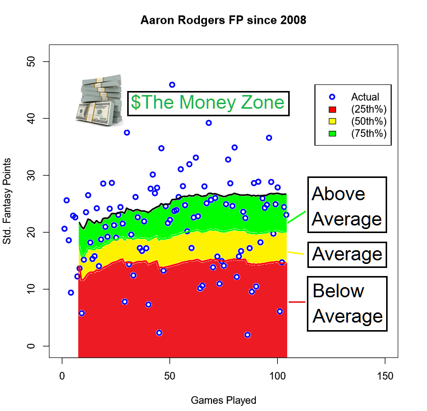
Above, I charted all of Aaron Rodgers Fantasy Performances since 2008, along with a rolling trend line of his 25th, 50th, and 75th percentile projections from the Gamma model for that given week. The vast majority of his performances fall in the Above Average zone. Not necessarily true of every player’s chart in the league, but this happens quite often for Mr. Discount Doublecheck.
Now, if this was just for your regular yearly fantasy league, I would probably just use the Q50 number as a reasonable estimate for each player. It is a pretty great middle across the board and errs on the side of underestimating a player’s performance, if anything. In yearly leagues, I just want to try and minimize my mistakes and avoid busts at all costs. I can deal with average performances.
Daily Fantasy Sports (DFS) is an ENTIRELY different animal. You MUST have the best possible player in every position on your team, subject to salary constraints of course. There is some art to this, there is some luck to this, but no matter what, you often have to try and shoot for the moon and go with a high risk high reward play. YOU HAVE TO PLAY TO WIN THE GAME!

Using the Q75 Assumption
So, with guns blazing, let’s use the Q75 as an aggressive estimate for our next week. How good does that do? Turns out, it’s pretty relative to the set of prior data you choose.
For example, in using 2008–2014 to predict 2015, I found many players were still positively influenced by past performances that had nothing to do with current performances. I call this the Chris Johnson, or CJ2K effect. He had a world beater 2008–2012 stretch. Then he sank like a stone. Granted he had a mild comeback last season, but my training data significantly overestimated his performances each week because it wanted 2009 CJ2K. What it got was consistent overestimate garbage.
So, as the saying goes often in data analysis, if garbage goes in, garbage comes out. And as I always say to my students in mathematical modeling - when in doubt, make a graph!
I’ve gone through many trials and tribulations, many time periods, and SO much math on my computer (just ask my wife, she loves me right now!).
I have found that in the end, a rolling two, maybe three year period of raw prior stats on a player is statistically sufficient and gives us the best chance to get some meaningful predictions using our Bayesian Modeling process going forward.
And by meaningful, I mean what gives me the best Coefficient of Determination (more on that to come).
Round of Plots Anybody?

Above represents every predicted NFL fantasy performance 2014–2015 (almost 8,000+ in total) using a players Gamma Q75, and the actual points they scored that week. The point (20, 40) on this plot means if I predicted they would score 20 that given week, they actually scored 40.
So great! we have a plot! What exactly does it all mean?
Well for one, its a lot of dots.
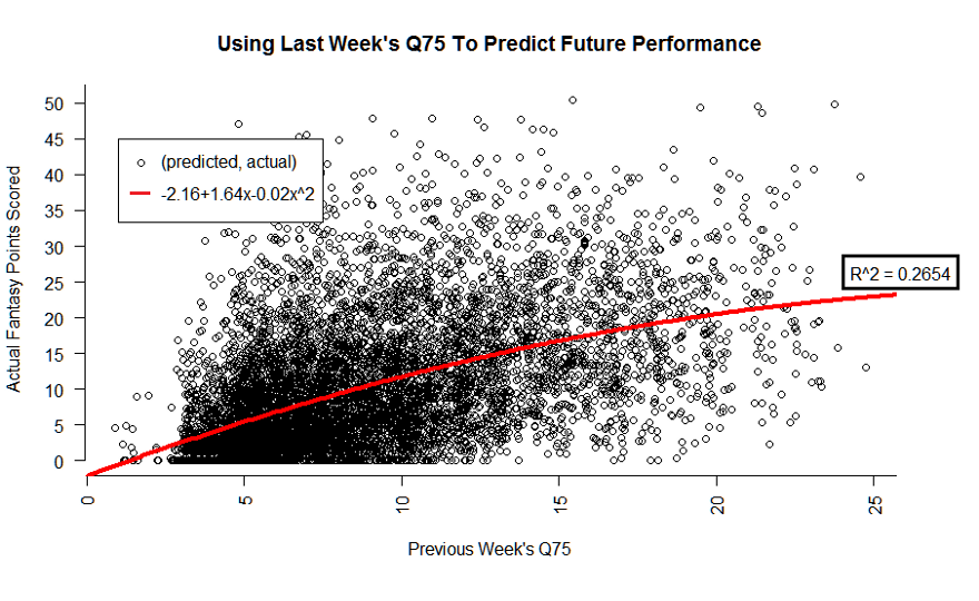
Past the obvious part, if our model was AMAZING, the dots would all be on a diagonal line where the previous week’s Q75 prediction would be precisely equal to the Actual Fantasy Points scored in the next week. My Algebra students out there may remember this as the line y = x. Something like this:
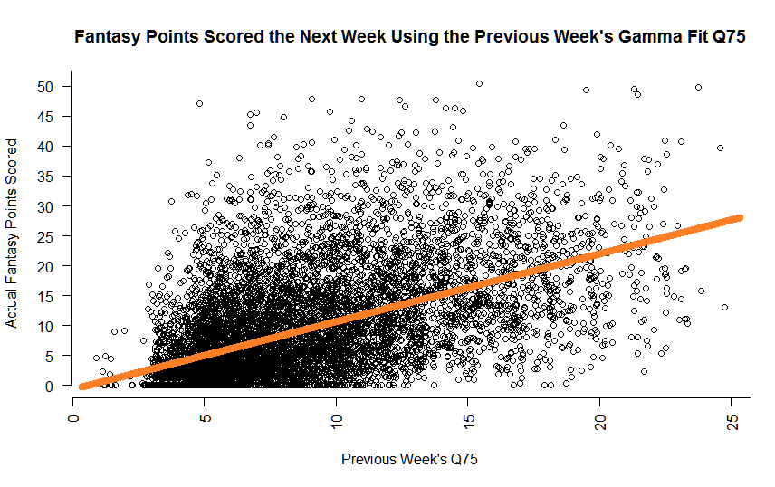
So our model is a teeny bit off from perfect. If you notice though, we have some promise. Our dots to the left are clustered closer to our orange “perfect” line, than the ones on the middle and the right. We might be able to explain this because players that tend to score low consistently, probably will not score high consistently in the future. These are your Fullbacks and Wide Recievers that are not likely to be used for more than 20 snaps a game. To stay with the Aaron Rodgers Packers theme, your John Kuhn’s of the world.
Your dots on the right are spread pretty wide from our line PRECISELY for the same reason we are going through this little exercise. BOOM OR BUST BABY! It is really REALLY hard to project breakout performances, especially just from a set of information related to one variable. That variable here, of course, being a player’s Gamma Q75 projection.
Goodness of Fit
Thankfully, there are better ways for us to perform this type of analysis instead of looking at a graph like it was a Banksy piece. We can perform what is known as regression testing!
If regression testing is something that makes you cringe, I sympathize. There was a time in my life where I seriously considered missing a college class on the subject because I hated it so much. I did miss that class, for the record, because my Inidina Hoosiers were in the NCAA Basketball Finals against Maryland. Priorities.
The cool thing is we don’t have to figure out any of this stuff by hand any more and the computers do it all for us. Yipee!
Linear Regression
Okay, we didn’t get a nice diagonal line to fit through our data. But, if we were to fit a line through our data that went through as many points as possible in our data set, what would that look line look like? Computer!
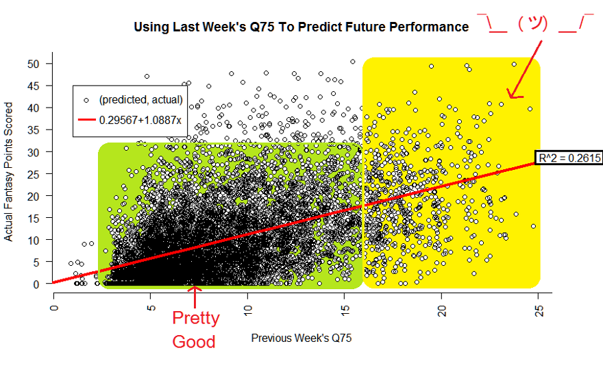
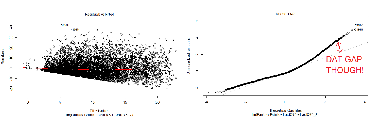
What does that mean for us exactly? As mentioned before, in the green zone we are still doing pretty well, but our line doesn’t account for much of our yellow zone. This is further backed up by the following residual charts:

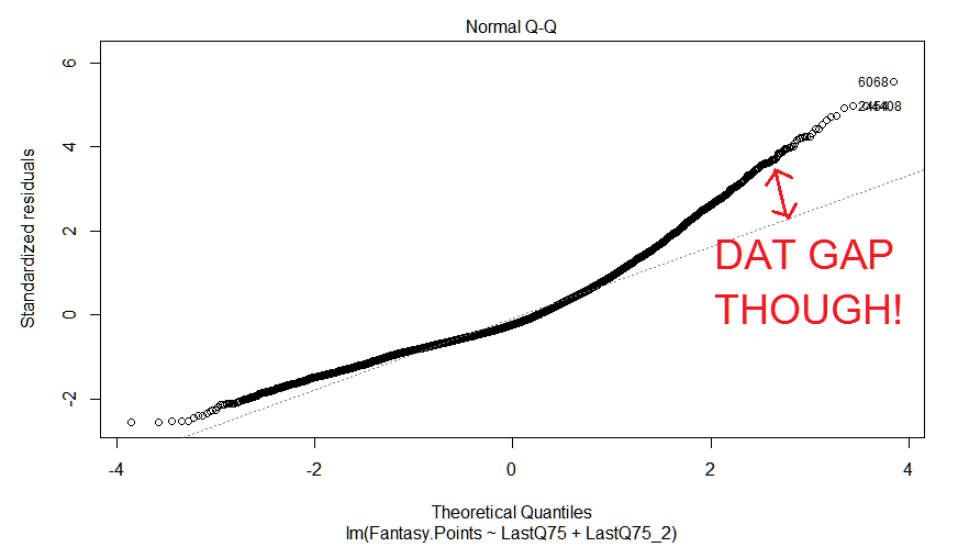
A residual is the difference between what our model predicts and what actually happened. Perfect would be 0, positive an overestimate, negative an underestimate.
On the left, you can see we tend to overestimate. But hey, isn’t that what we tried to do here in the first place by being so aggressive with our Q75 choice?
The graph on the right is basically a different way to view this information in terms of the spread of our residuals. Are our residuals are nicely spread apart, or do they deviate severely from our perfect zero? We want to be on the diagonal line on this plot. Our biggest gap is to the right, with our high predicted point value players, as predicted prior.
The Devil is in The Details
Below is the summary of our linear regression. Notice here that even though we were spread apart, our LastQ75 is rated by the computer as mattering, meaning it does have high significance towards explaining the randomness of a future fantasy performance. How much so? Basically 26%.
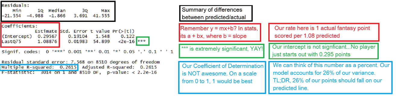
Now, before you queue up the Price is Right loser horn, 26% really is not that bad. If you think about it, we have a way to account for at least a quarter of the randomness that happens week to week in football. This is pure chaos folks, and we have eaten two slices of that pizza!
Our main goal now would now be to come up with other factors that might influence variance. Specifically, variance at the upper level of the spectrum. WE WANT TO CATCH THESE FANTASY WHITE WHALES!
Other Types of Regression
If you’ve made it this far, either I’m a really good writer, or you are a stat head. Either way, you deserve to know there are other regressions out there. Maybe a line doesn’t fit our data well, maybe it’s another type of curve?
You better believe I’ve performed these regressions too. Oh yes, I’ve performed them alright. Here’s a few greatest hits.
Quadratic Regression
Uses a bowed parabola curve to fit the data instead of a line. You know, parabola? Your nightmare from Algebra 2?
We have a marginally better R^2 value here, increasing our accuracy by less than half a percent. The residuals?
Exponential Regression
Uses a exponential curve (think the Nike swoosh) to fit the data instead of a line. I must admit, I was excited before I performed this test because of its potential to fit our high end data. I ended up here with a big bowl of meh.
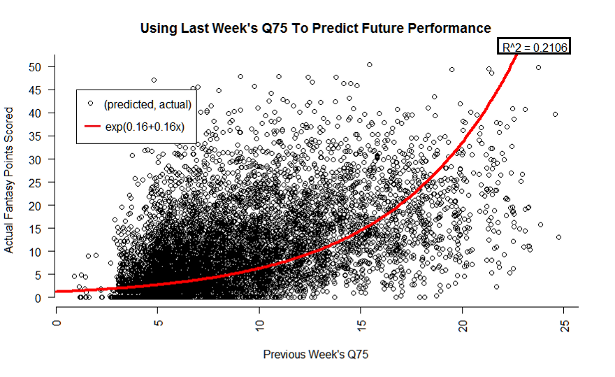
So, we fit our upper data pretty well at the sacrifice of the lower end. COMPUTER, residuals!

What does this all mean?
It means that while we have the start of a really good model, we have some gaps to fix. Our models were each significant, in that we know past performance with our Bayesian thinking does have an effect on future performance. We just know it can only account for about a quarter of the variance that happens with games at best.
We are just taking in one variable only to predict future performance. Perhaps there are more out there that we are not considering and would make an excellent addition to our model. I will investigate all this and more in my next part!