Hi. I wanted to play around with linear algebra Python, and the Numpy package. In the past, I have used MATLAB for linear algebra work but nowadays MATLAB does not seem like a viable option with Python's Numpy package being around.
Sections
- Some Vector Operations
- Some Matrix Operations
- References
Some Vector Operations
Creating Vectors
To start, here are two vectors a = (1, -3, 5) and b = (2, -1, 7).
>>> ## Vectors:
...
... a = np.array([1, -3, 5])
... b = np.array([2, -1, 7])
...
... print(a)
... print(b)
[ 1 -3  5]
[ 2 -1  7]
Vector Addition
With vector addition and vector subtraction, it operates element-wise.
>>> print(a + b) # Vector addition
... print(a - b) # Vector subtraction
[ 3 -4 12]
[-1 -2 -2]
Scalar Multiplication
Here is an example of scalar multiplication on a vector.
>>> print(2*a) # Scalar multiplication on vector
[ 2 -6 10]
Dot Products Of Vectors
Given two vectors (of equal size), one can compute the dot product of the two vectors.
>>> # Dot Product (Element wise multiplication and take sum of products):
...
... print(np.dot(a, b)) # (1*2) + (-3)(-1) + 7*5 = 2 + 3 + 35 = 40
40
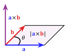
Cross Products Of Vectors
The cross product of two vectors is a (third) vector that is perpendicular/orthogonal to both vectors. (i.e. The z-axis is orthogonal to both the x-axis and the y-axis.)
>>> # Cross Product (A Vector That Is Perpendicular/Orthogonal To Vectors a and b):
...
... cross_vect = np.cross(a, b)
... print(cross_vect)
[-16   3   5]
Using Dot Products To Check Orthogonality
To make sure that this (-16, 3, 5) vector is indeed orthogonal to the vectors a = (1, -3, 5) and b = (2, -1, 7) the dot product is used. If the dot product is zero between two vectors, then those two vectors are orthogonal to each other.
# Check orthogonality by seeing dot product is zero between cross product with a and b:
...
... print(np.dot(cross_vect, a))
...
... print(np.dot(cross_vect, b))
[-16   3   5]
0
0
Math Function Example
Here is an example with a math function. I have a list of x-values being 0, 1, 2 and 3. These x-values are inputted into the exponential function.
>>> # Function example:
...
... x = np.array([0, 1, 2, 3])
...
... print(np.exp(x))
[  1.           2.71828183   7.3890561   20.08553692]
Random Number Generation Example
Random numbers can be generated element-wise. In this example, I generate random numbers from a normal distribution.
>>> # Vector with random numbers from a normal distribution.
...
... print(np.random.normal(size = (1, 4)))
[[-1.87577226 -0.77085276 -0.39107313  0.36635035]]
Some Matrix Operations
Special Matrices
To start this section, here are some special matrices such as the identity matrix, the matrix with zeroes and the matrix of ones.
>>> ## Matrices:
...
... # 5 by 5 Identity Matrix
...
... identity_five = np.identity(5)
...
... print(identity_five)
[[ 1.  0.  0.  0.  0.]
 [ 0.  1.  0.  0.  0.]
 [ 0.  0.  1.  0.  0.]
 [ 0.  0.  0.  1.  0.]
 [ 0.  0.  0.  0.  1.]]
>>> # 3 by 3 Matrix of zeroes:
...
... print(np.zeros( (3, 3)))
...
[[ 0.  0.  0.]
 [ 0.  0.  0.]
 [ 0.  0.  0.]]
>>> # 3 by 3 Matrix of ones:
...
... print(np.ones( (3, 3)))
[[ 1.  1.  1.]
 [ 1.  1.  1.]
 [ 1.  1.  1.]]
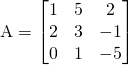
Creating A Matrix In Numpy
Creating a matrix in Numpy can be confusing. You may ask yourself, which one is a row and which one is a column. Matrix rows are represented by the lists inside the one list. In the example below, the first row has the elements 1, 5 and 2, the second row has 2, 3 and -1 and the third row has 0, 1 and - 5.
>>> # Creating a matrix:
...
... A = np.array([[1., 5., 2.], [2., 3.,-1.], [0., 1., -5.]])
...
... print(A)
[[ 1.  5.  2.]
 [ 2.  3. -1.]
 [ 0.  1. -5.]]
Determinant Of A Matrix
Given a square matrix, the determinant can be determined with the det() function from the linear algebra package.
>>> # Matrix determinant:
...
... det_A = np.linalg.det(A)
...
... print(det_A)
...
40.0
Diagonal Of A Matrix
The diagonal of a matrix consists of the numeric entries along the main diagonal. In matrix A, we have 1, 3 and -5.
>>> # Diagonal of Matrix:
...
... print(np.diag(A))
[ 1.  3. -5.]
Trace Of A Matrix
The trace of a square matrix is the sum of the matrix's diagonal entries. From matrix A, the trace would be 1 + 3 - 5 = -1.
>>> # Trace Of A Matrix:
...
... print(np.trace(A))
-1.0
Transpose Of A Matrix
The transpose of a matrix has the rows and the columns switched.
>>> # Transpose Of Matrix:
...
... print(np.transpose(A)) # Transpose of matrix A
...
[[ 1.  2.  0.]
 [ 5.  3.  1.]
 [ 2. -1. -5.]]
Inverse Of A Matrix
>>> # Inverse Of A Square Matrix:
...
... print(np.linalg.inv(A))
[[-0.35   0.675 -0.275]
 [ 0.25  -0.125  0.125]
 [ 0.05  -0.025 -0.175]]
Matrix Multiplication
Matrix multiplication involves at least two matrices and operates differently than typical multiplication. In math notation, I have:
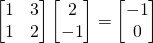
>>> # Matrix multiplication:
...
... B = np.array([[1, 3], [1, 2]]) # 2 by 2 matrix
...
... D = np.array([[2], [-1]]) # 2 by 1 matrix
...
... print(np.matmul(B, D))
[[-1]
 [ 0]]
Solving Linear Systems
Linear algebra is useful when it comes to solving linear systems. In this example, we seek values of x1 and x2 such that they satisfy the equations.
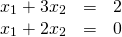
The above system of equation can be expressed in linear algebra form like this:
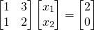
The linear system can be solved in Python's Numpy with the solve() function.
>>> # Solving a linear system example Bx = c.
...
... B = np.array([[1, 3], [1, 2]])
...
... c = np.array([[2], [0]])
...
... print(np.linalg.solve(B, c))
[[-4.]
 [ 2.]]
The solutions would be x1 = -4 and x2 = 2. (since -4 + 6 = 2 and -4 + 4 = 0).
References
- Python For Data Analysis Book (O'Reilly Media)
- https://docs.scipy.org/doc/numpy-dev/user/quickstart.html
- https://docs.scipy.org/doc/numpy/reference/routines.linalg.html
- Other Scipy documentation.