In this article we will forecast the Bitcoin price until 2018 and see what the probability range is to hit the 1000$. In the last article we've talked about Bitcoin probability distribution, but since it cannot be accurately applied to a price chart, we have to rely on time series.
If you missed the first part, you should read it, so you will know what I am talking about:
@profitgenerator/let-s-calculate-the-probability-of-bitcoin-going-to-1000usd-and-above-pt-1
Any price series is a time series, because it's a 2 dimensional probability plane. On one hand you have the probability distribution of the price, and on the other hand you have the time factor. Therefore the variance is not static, neither is the average price. We call this phenomena Heteroscedasticity.
Therefore in Time Series Analysis we use regressive and moving average models to calculate the "moving average", and the "moving variance". One method is ARMA.
AR-MA
The ARMA model is composed of an autoregressive part and a moving average part. I have successfully found my old quant python scripts on my old hard-disk so I did a few calculations yesterday.
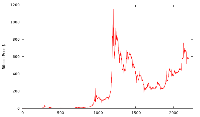
I have again used the Bitcoin price data in $, via Blockchain.info, and this is how the full Bitcoin price looks plotted:
Now we have to calculate the ARMA, but before that we need to find the right p and q coefficients, or ranks. The p is the coefficient of the AR (autoregressive) part, and the q is the coefficient of the MA (moving average) part.
We use a Partial autocorrelation function with at least 70 degrees of lags, and we observe that the value 1 has the highest correlation with the data.
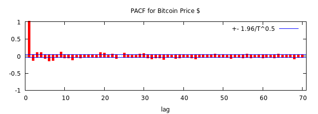
Therefore the p and q values will be 1. Now of course we still need to do additional tests to verify this, but more on that later. So we have ARMA (1,1) as a good tool for the Bitcoin price.
We calculate ARMA (1,1) which will have the following properties:
| variable | coefficient | std. error | z | p-value |
|---|---|---|---|---|
| constant | 274.383 | 139.732 | 1.964 | 0.0496 |
| phi | 0.997582 | 0.00147242 | 677.5 | 0.0000 |
| theta | 0.155137 | 0.0217816 | 7.122 | 1.06e-12 |
Then we test the errors, which is the most important part:
| Mean Absolute Error | 6.477 |
|---|---|
| Mean Percentage Error | -200.15 |
| Mean Absolute Percentage Error | 202.17 |
| Mean Error | -0.010629 |
| Mean Squared Error | 265.88 |
| Root Mean Squared Error | 16.306 |
Of which I think the MAE is the best benchmark, as the MSE and the RMSE is very biased since a lot of root squaring is going on. An error of 6.477 is still pretty big, so your accuracy will be as high as much you can reduce these values.
It will never be 0, since there is a lot of random noise, and missing information (the price goes on forever), but if you can reduce this as much as possible, you will have better forecast results.
Let's plot the ARMA(1,1) on the chart, and compare:
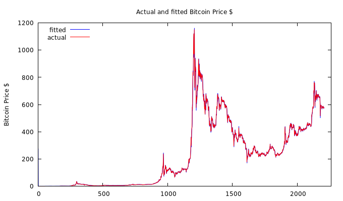
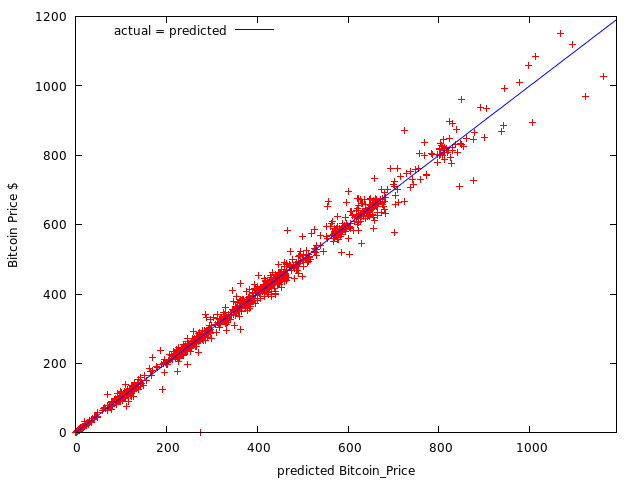
As you can see it fits almost perfectly, if not for that error. Now let's extrapolate our model, and forecast with 70% probability range, the price until 2018:
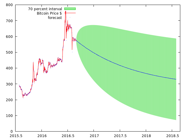
And as you can see the ARMA(1,1) model predicts are disaster for Bitcoin, it does not reach the 1000$ ever and it has a big chance of going to 0$.
But don't panic, because the ARMA model is not the best model for the Bitcoin price, and in fact it's not even very accurate. The Bitcoin price has a trend, and we need to difference the price until the trend is eliminated, so we have to use another model.
AR-I-MA
ARIMA is an parent model for the ARMA, and it has an extra variable for differencing. Technically our ARMA (1,1) is an ARIMA (1,0,1) where we have 0 orders of differencing. We have to integrate the model to reduce the non-stationarity, the trend.
Now a trend can clearly be seen in Bitcoin, but how to quantify that? It is pretty subjective. We use an Augmented Dickey–Fuller test to measure the strength of the trend.
I have tested all variants of the ADF test, and the following p-values have been given:
Augmented Dickey-Fuller test for Bitcoin_Pricetest with constantasymptotic p-value 0.4856with constant and trendasymptotic p-value 0.3379with constant and quadratic trendasymptotic p-value 0.5702test without constantasymptotic p-value 0.2972It's a general rule of thumb, if p is bigger than 0.05, we have a trend, and we have proven this objectively.
Therefore we calculate an ARIMA (1,1,1), we already know p and q is 1, and we assumed d = 1.
| Mean Absolute Error | 6.2399 |
|---|---|
| Mean Percentage Error | -15.478 |
| Mean Absolute Percentage Error | 17.756 |
| Mean Error | 2.8442e-05 |
| Mean Squared Error | 231.87 |
| Root Mean Squared Error | 15.227 |
Now our MAE is much smaller and the other error benchmarks too, which will indicate a better chance of success. Now we forecast the Bitcoin price until 2018 with ARIMA(1,1,1) and with 70% boundaries:
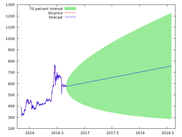
See the difference? ARIMA(1,1,1) is much more accurate than ARMA(1,1) for the Bitcoin price, and it shows completely different results.
Now we can say that Bitcoin has a 70% chance of being in the green boundary in the next 2 years. And it has less then 30% chance of going under 300$, which is good, very good!
Now let's tweak it a bit, and do an ARIMA(1,2,1):
| Mean Absolute Error | 6.1974 |
|---|---|
| Mean Percentage Error | -0.43986 |
| Mean Absolute Percentage Error | 3.5761 |
| Mean Error | 0.020351 |
| Mean Squared Error | 233.18 |
| Root Mean Squared Error | 15.27 |
Even smaller errors, so our forecasting accuracy will be very much improved. We plot ARIMA(1,2,1) with 60% boundaries, until 2018:
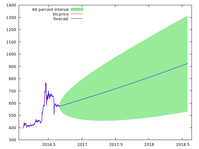
So there is a 60% of the price being inside, and a 40% of the price being outside the boundaries. But also the slope has changed and it shows an even more optimistic future for Bitcoin.
We know that ARIMA(1,2,1) is more accurate since it has less error margin, and we have an even higher area covered, possibly until 1300$.
The ARIMA shows that the 900$ could be hit at 2018 with average luck, but any estimation beyond that becomes degraded, as the more you forecast into future, the less accurate it becomes.
If we continue with this pace, the Bitcoin price has a good probability to become 1000$ in early 2018.
Thanks for reading through, if you've liked this article series, please show it by upvote. If I get many upvotes, I will talk more about econometrics, quantitative analysis and forecasting prices!
Disclaimer: The information provided on this page might be incorrect. I am not responsible if you lose money from the information you've read on this page! This is not an investment advice, just my opinion and analysis.
Title Image from: https://pixabay.com