With this post, I am carrying on with the export of my CERN particle physics lectures at a level where anyone on Steemit could get something out of them.
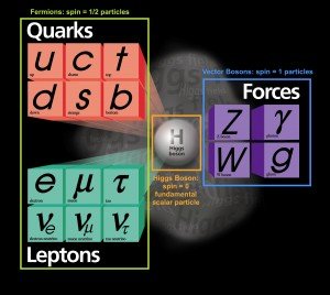
I recall that I have introduced all the elementary beasts we are interested in in this first post.
The summary is shown on the picture below, the matter particles being shown on the left, the interaction mediators on the right and the Higgs boson allowing for explaining the particle masses in the middle.
 [image credits: Fermilab ]
Now it is time to describe the equations driving the Standard Model of particle physics and detail what practical calculations can be done with these equations. I will concentrate on particle production rates at the CERN Large Hadron Collider (LHC), which will lead to a first insight into the challenges for discovering new physics at particle colliders.
The outline of this post is:
- The Standard Model Lagrangian
- Colliding protons at the LHC
- Total production rates
- Standard Model cross sections - part I
- Standard Model cross sections - part II
- LHC analyses
- Summary
[image credits: flickr and quantum diaries]
THE STANDARD MODEL LAGRANGIAN
The equations driving the interactions among all elementary particles can be derived using symmetry principles and quantum field theory.
Without entering into any technical detail (see this post of @nonlinearone for an appetizer), the take-home message is that those symmetries allow one to define a basic compact object containing all the physics, the Standard Model Lagrangian.
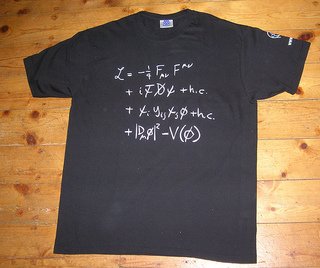
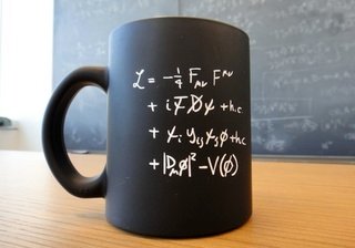
The Standard Model Lagrangian turns out to be sufficiently compact so that it fits either on a t-shirt or on a mug (that can be bought at CERN). See the above pictures.
By the way, there is a mistake on the equation shown on these goodies… One h.c. too much on the second line ;)
Once expanded (each symbol of the Lagrangian contains many stuff in it), the Standard Model Lagrangian consists of hundreds of terms dictating the way in which the elementary particles propagate in spacetime and interact with each other (via strong, weak and electromagnetic interactions).
 [image credits: BNL]
COLLIDING PROTONS AT THE LHC
How to make a calculation with the Standard Model Lagrangian?
The best way to answer this question is to take an example. In the rest of this post, I will only consider proton-proton collisions such as occurring at the CERN LHC.
When one considers a specific proton-proton collision at the LHC, one can calculate, with the help of the Standard Model Lagrangian, the probability with which two protons will annihilate into a given final state.
For instance, one can compute the probability with which a Z-boson or a Higgs boson will be produced from the annihilation of two protons.
That could be chocking on a first sight, but quantum theories are probabilistic.
In our case, there are different options for the result of a given collision, and the only thing that one can calculate is the probability with which each of these options could be realized.
It is hence not possible to exactly predict the result of a given LHC collision and one must restrict ourselves to the calculation of the probability with which each possible result will occur.
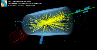 [image credits: Fermilab]
TOTAL PRODUCTION RATES
Inversely, having a definite number of LHC collisions, one can derive the mean number of collisions that will give rise to any specific final state.
The key quantity for this derivation is the production rate associated with the process under consideration, or in the jargon of particle physics, the corresponding total cross section.
Now, taking the bestiary of particle physics presented in my previous post, there is an infinite number of Standard Model processes that could be studied:
- proton-proton annihilating into one Higgs boson (or more);
- proton-proton annihilating into a pair of weak bosons (or more);
- proton-proton annihilating into two or more top quarks;
- proton-proton annihilating into almost any combination of particles we may think of.
These processes are however not all relevant. Some cross sections are indeed so small that even after 25 years of LHC running, they will not give rise to anything observable despite the fact that hundreds of millions of LHC collisions occur each second.
For instance, it is very unlikely that any triple-Higgs event (a collision leading to a final state comprised of three Higgs bosons) will be observed.
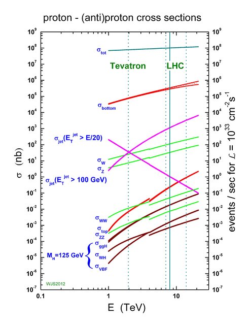
The cross sections for the most relevant Standard Model processes (with the largest cross sections) are shown in the picture below. Please do not run away (or close the webpage), I now explain everything that is on this figure.
 [image credit: James Stirling]
STANDARD MODEL CROSS SECTIONS - PART I
There is a lot of information on the above picture.
First of all, the x-axis corresponds to the collision energy.
There are several vertical lines and I will only focus on the rightmost dashed line that correspond to the current collision energy at the LHC.
Next, there are two y-axes on the figure, one for the cross section (left-hand side) and one for the corresponding number of events per second (right-hand side). Those two quantities are proportional to each other, and for the sake of clarity, I will only discuss the event rate.
I recall that an event of a specific type is a collision giving rise to this specific final state. A top-antitop event consists thus of a collision in which a top quark and a top antiquark are produced in a proton-proton collision.
Moreover, an event rate only means something for a given LHC luminosity, or a given number of LHC collisions per second. The number chosen here equals one tenth of the current number of LHC collisions per second.
To summarize with an example, let us take the lowest red line. This line is related to collisions in which at least one top quark is produced. Checking the intersection with the rightmost vertical line, this means that one can expect, for the chosen luminosity, one top event per second.
[image credit: James Stirling]
STANDARD MODEL CROSS SECTIONS - PART II
Now we can investigate the figure.
The upper dark green line represents the LHC total cross section, i.e., the number of events where a proton-proton collision has produced something. Any other line represents an interesting Standard Model process.
Checking the y-axis numbers, only 1% of the collisions that produce something are connected to interesting Standard Model physics!The purple lines are related to jet physics. This equivalently concerns the production of quarks and gluons at the LHC, which gives rise to jets containing a large number of particles thanks to quantum chromodynamics (I will skip any further detail here).
The production of jets has hence a very large probability to occur. The associated rate is nevertheless already very suppressed as soon as we compare the numbers to the total cross section value.The red lines are related to the production of third generation quarks (top and bottom quarks).
The top quark is the last quark that has been discovered (in 1995), and the LHC is a top quark factory: one top quark is produced every second (for the chosen luminosity). The difficult task left to experimentalists is to observe this top event within the 100.000.000 other events that are produced every second.The light green lines are related to electroweak physics, or to the production of one or more than one W or Z bosons.
Finally, the brown lines are related to Higgs physics.
Any new physics process would correspond to a cross section even smaller (to be added on the right-lower corner of this figure). However, nature may be nasty so that not a single new physics process would be observable at the LHC.
But that is all what exploration is about: we explore and we do not know what will be found.
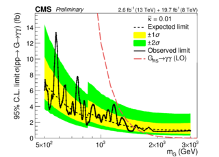 [image credit: inspire ]
LHC ANALYSES
The cross section figure that we have just described shows that interesting events are rare.
For instance, 1 new physics event (our signal of interest) will be, in the best case scenario, hidden within 1.000 Higgs boson events and 1.000.000.000.000 Standard Model events (both constitute the background).
The signal of yesterday (the Higgs boson) is thus the background of tomorrow.
That is actually always the case: top quark events were the most searched signal events in the nineties. They are today one of the most painful background to get rid of.
And this is what LHC analyses are about: reduce the background as much as possible without throwing away the signal.
The way to do that is to impose restrictions on the topology of the events to consider.
For instance, one may veto events exhibiting the presence of this or that particle in the final state, or impose that the energy of this or that final state particle is above some threshold.
Those selections reduce the cross section, and the goal of each LHC analysis is to find good selections killing the background without affecting the signal (too much).

SUMMARY
In this post, I have discussed the core quantity of the Standard Model of particle physics, its Lagrangian describing the way in which particles propagate in spacetime and interact with each other.
Taking the example of the LHC, I have then introduced the concept of a cross section, a quantity that can be calculated from a Lagrangian and that is related to the production rate of a given process at the LHC.
I have finally investigated the LHC production rates of the most relevant Standard Model processes and sketched the challenges associated with an LHC analysis: new physics is like looking for a needle in a needle stack.