Image Processing - Stacking
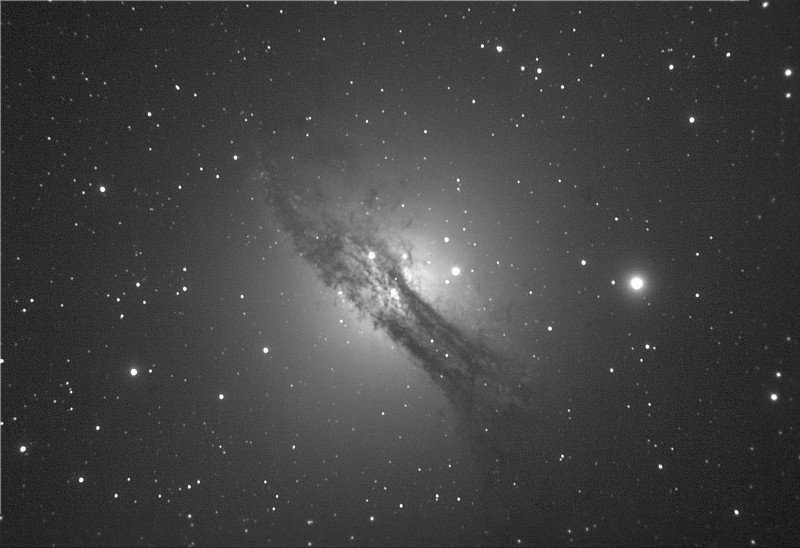
Active Galaxy Centaurus A imaged by the author. To obtain this image 1370 exposures of 4 seconds were stacked using the summation method
In the previous part of this series (part 8), I examined a typical astronomical image processing workflow as shown in the following diagram.
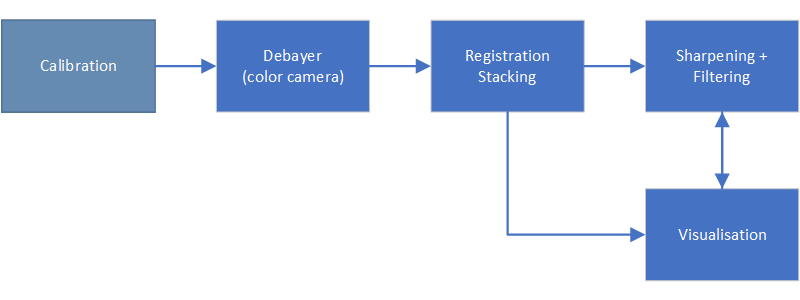
Now we shall look at stacking (step 3 in the workflow), as well a bit of background on why it works (and why astronomers love image stacking!).
Intro
Image Stacking is the technique of creating a single composite image from multiple photos of a subject. There are several common methods of stacking which we look at in this article. At the end of this blog I will talk more in depth with some theory, but the next section is more the practical application.
Stacking Methods
Summation and Averaging
The summation method creates a composite image using addition to combine the images. In Photoshop or Gimp, this would be equivalent to placing the images on separate layers and setting the layer mode to addition.
Summation method of stacking, showing the stacking of 4 images. The image has been displaced topographically proportional to pixel brightness
This method is very fast but it's Achilles heel is if one the images have a flaw this will be visible in the final stacked image. This flaw could be anything from an aircraft flying through the frame to a cosmic ray strike on the sensor.
Example : Here is an example of stacking a sequence of 16 individual photos of galaxy NGC4945. Here is a screen capture of the thumbnails for each of the photos. Note that the last photo 'Capture_0016.fit' has an aircraft trail through the bottom left and we will see how we can deal with this.
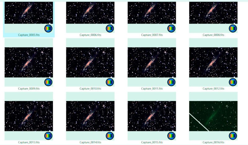
This is the image list thumbnails used to generate the example stacked image (see below)
For reference here is what a single image looks like. You can see the background is quite noisy.
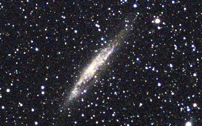
Single photo 'Capture_0001.fits' from above Sequence shown full size
When the 16 photos above are stacked using the summation method the following image is the result. Note the noise is much less and a lot more detail is now present. However, note that the aircraft trail from photo Capture_0016.fits unfortunately still shows in the stacked image. This is the major downside to this method of stacking.
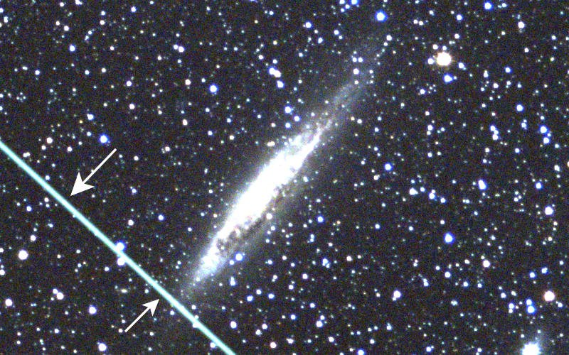
Summation stacking of 16 images. Notice how much better the image is compared to the single frame above, although unfortunately the aircraft trail present in image number 16 is clearly visible
Median
If a median method is used instead of summation, the rejection of flaws in a single image is greatly improved. The median method takes the statistical median value of the images to obtain the stacked image.
The following image is a median stack using the same image set as the one used for the previous image. Notice that the trail is almost gone (only a faint trace can be seen). The median stacking method is much slower than summation and it may be just as effective to remove the flawed image from the image stack if the number of photos is large.
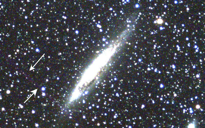
Median stacking of 16 images
Sigma Rejection
The Sigma Rejection method of stacking removes any pixel values in the photo stack that are very different in brightness from the other pixels. It does this by using the standard deviation of the pixel values, and removing any values too far from the mean.
Sigma Rejection is best at removing single frame flaws in an image stack, as can be seen in the following example where the 16 photos have been combined using this method. Note the aircraft trail is now completely invisible.
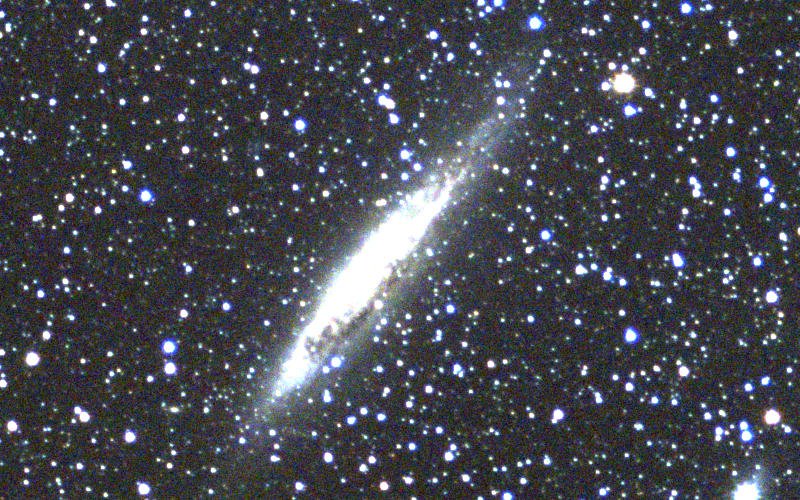
Sigma Rejection stacking of 16 images
Theory and Background
Image
An image is represented in a computer by an array or matrix of pixels as shown in the following diagram. Each pixel in the array is referenced by specifing the row and column position. The pixel value represents the brightness of the image at that point. For color images the array pixels will also contain the brightness for red, green and blue which is stored in memory as a single 24,48 or 96 bit value.
![]()
A typical image can be considered to be an array or matrix of brightness values as shown here. Pixels are referenced by a column and row index number
Summation Stacking
The simplest form of image stacking is summation where the pixel values at each pixel position (specified by row and column) are added together across all of the images. In mathematically terms the operation can be described as follows:
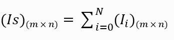
Where IS is the stacked image array and Ii is a sequence of N image arrays to be added. m x n refers to an image array of width x height
Signal to Noise Ratio (SNR)
When images are summed together correlated information such as stars and galaxies will generate a signal in direct proportion to the exposure time. Therefore by doubling an exposure all the stars in the image will register twice the signal. By correlated, we refer to any signal source that is persistent across all the images in a stack.
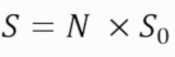
Where S is the total signal of an object, N is the number of the exposures and S0 is the signal of an object in a single exposure
In real images, random noise is almost always present. Even if the camera is perfect and introduces no noise of its own, light itself generates noise (called shot noise) and this is not correlated from one image to the next. One property of this noise is that it does not add proportionally in stacking. In fact, noise sources combine together as follows:
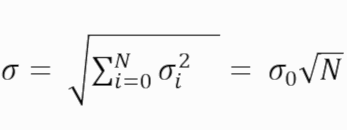
Where σ is the total noise in the image stack, N is the number of the exposures and σ0 is the noise in a single exposure
Real images contain random noise (uncorrelated information) and detail (correlated information). When you combine them you get the real image on the right
Once we know the signal and once we know the noise level, we can compute Signal to Noise (SNR) as just S / σ. Typically, for basic detection SNR > 3 and for highly confident detection SNR > 5. If we just wish to compute the improvement in SNR due to stacking we can calculate it as follows:
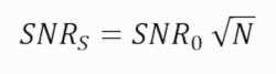
Where SNRs is the SNR of the image stack, N is the number of the exposures and SNRσ0 is the SNR of a single exposure
Hence in the image in title, 1370 images were added in the stack. This should have resulted in an improvement of 37 times in image quality over a single image. Now you know why astronomers love image stacking!
Why can't I stack the same Image?
Some people have asked why can't one just stack the same image over and over again. The reason is all the detail and noise in the image is correlated between the images, so there is no net gain in SNR.
Observations versus theory
It is interesting to see that those above predictions work very well in practice. We can actually measure this. The following data shows actually measurements that were made off the photos made in the earlier examples.
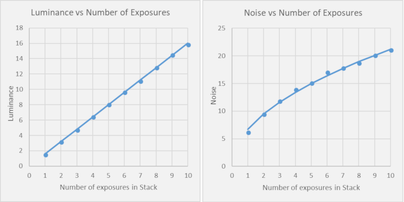
Actual measurements (point markers) versus Theory (solid line). Observation is indeed consistent with predictions!
Conclusions
In this article, we looked at a couple of different methods for image stacking (as well as some theory). We saw how effective stacking was in improving image quality. Next time around I will be looking at filters with a few examples to show you just how effective they can be at improving images.
References
- Buil, Christian. CCD Astronomy: Construction and Use of an Astronomical CCD Camera. Richmond, VA: Willmann-Bell, 1995.
NOTE: All images in this article are the author's, please credit @terrylovejoy if you wish to use any of them.