Particle physics @ utopian-io - Objects isolation, histogramming an...

This series of posts aims to offer a way to developers to contribute to state-of-the-art research in particle physics through the reimplementation, in the MadAnalysis 5 framework, of existing searches for new phenomena at the Large Hadron Collider, the LHC, at CERN.

The grand goal of this project is to extend the MadAnalysis 5 Public Analysis Database. The analyses included in this database are used by particle physicists to assess how given new particle physics theories are compatible with the observations at the LHC.

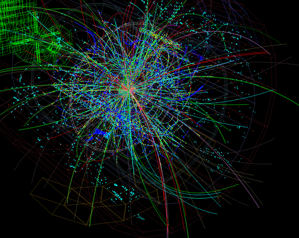
_{[image credits: Pcharito (CC BY-SA 3.0)]}

Among all the concepts introduced so far (please have a look to the end of this post for a table of content), the most important one consists in the notion of events.

An event can be seen as a record in an LHC detector, originating either from a real collision or from a simulation.

Roughly speaking, such events contain a set of objects reconstructed from various hits and tracks left in the detector.

We have for now discussed four of these objects, namely photons, electrons, muons and jets. In parallel with the physics, we have also detailed how to access those objects and their properties in the MadAnalysis 5 framework.

At the end of the last episode of this series, we have introduced the removal of the potential overlap between different objects.

In this post, we will move on with object isolation, and then tackle a totally different topic and discuss how the MadAnalysis 5 framework can be used for histogramming. In other word, I will describe how to focus on a specific property (of an object or even the entire event) and represent it in a figure (a histogram).

This post will end up with a traditional exercise. We will today, for a change, focus on a search for dark matter performed by the CMS collaboration.

A first task request will also be proposed, targeting the development of a new add-on to MadAnalysis 5.

SUMMARY OF THE PREVIOUS EPISODES

_{[image credits: geralt (CC0)]}

In the first post on this project I explained how the MadAnalysis 5 framework could be downloaded from LaunchPad or GitHub.

Moreover, I have also detailed how any necessary external dependencies could be downloaded and linked.

In the next two posts (here and there), we have started dealing with the real work.

I have discussed in some details the nature of four of the different classes of objects that could be reconstructed from the information stored in a detector. Together with their representation in the MadAnalysis 5 data format, those are:

Electrons, that can be accessed through event.rec()->electrons(), that is a vector of RecLeptonFormat objects.
Muons, that can be accessed through event.rec()->muons(), that is a vector of RecLeptonFormat objects.
Photons, that can be accessed through event.rec()->photons(), that is a vector of RecPhotonFormat objects.
Jets, that can be accessed through event.rec()->jets(), that is a vector of RecJetFormat objects.

We have in parallel started to investigate the main properties of those objects (let us take a generic one called object), namely their transverse momentum (object.pt()), transverse energy (object.et()) and their pseudorapidity (object.eta() or object.abseta() for its absolute value).

The transverse momentum is related to the component of the motion of the object that is transverse to the collision axis. Similarly, the transverse energy consists in the energy deposited transversely to the same axis, and the pseudorapidity describes the object direction with respect to the collision axis.

Because of the remnants of the colliding protons, anything parallel to the collision direction is too messy to get any useful information out of it. For this reason, one restricts the analysis to what is going on in the transverse plane.

In addition, I have introduced the angular distance between two objects object1 and object2 (object1.dr(object2)) that allows us to assess how the two objects are separated from each other. This allows to lift any potential double counting occurring when the same detector signature is tagged as more than one object.

Along these lines, it is good to know that MadAnalysis 5 works in such a way that one must always remove the overlap between electrons and jets. Assuming that one has a jet collection named MyJets and an electron collection named MyElectrons, one must include into the code:

   MyJets  = PHYSICS->Isol->JetCleaning(MyJets,  MyElectrons, 0.2);

This automatically clean the jet collection from any electron candidate.

ISOLATION

The identification, or reconstruction, of the physics objects leaving tracks in a detector is crucial. Any analysis is indeed based on imposing some requirements on those reconstructed objects, so that identifying good-quality reconstructed object is therefore crucial.

For this quality reason, one often requires the objects of interest to be well separated from each other. In other words, one imposes some isolation criteria.

One easy way to implement object isolation is to rely on the angular distance between different objects. For instance, we may impose that no object is reconstructed at a given angular distance of a specific object of interest. Implementing such an isolation is easily doable with the methods yielding object overlap removal (see my previous post).

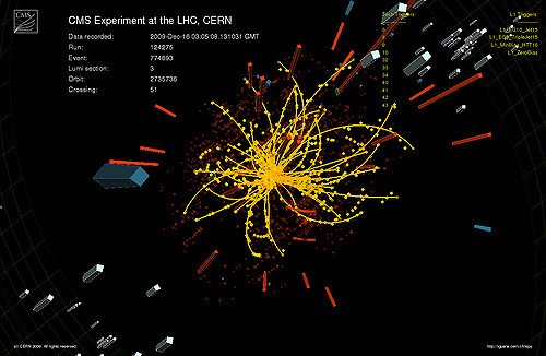
_{[image credits: Todd Barnard (CC BY-SA 2.0)]}

However, there is another, very widely used, way. Let us take for instance this CMS search for dark matter. This analysis relies on the presence of an isolated photon.

Such an isolated photon is defined as a photon for which there is not much activity around it.

In order to assess quantitatively this activity, we consider a cone of a given radius dR centered on the photon.

One next calculates three variables I_π, I_n and I_γ, related to the sum of the transverse momenta of all charged hadrons, neutral hadrons and photons present in the cone respectively. In other words, one considers all charged hadrons, neutral hadrons and photons lying at an angular distance smaller than dR of the photon.

Those sums are finally compared to the transverse momentum of the photon. If they are relatively small enough, the photon will then be tagged as isolated.

MadAnalysis 5 comes with predefined methods allowing to calculate those sums,

   double Ipi = PHYSICS->Isol->eflow->sumIsolation(myphoton,event.rec(),0.3,0.,
      IsolationEFlow::TRACK_COMPONENT);
   double In = PHYSICS->Isol->eflow->sumIsolation(myphoton,event.rec(),0.3,0.,
      IsolationEFlow::NEUTRAL_COMPONENT);
   double Igam = PHYSICS->Isol->eflow->sumIsolation(myphoton,event.rec(),0.3,0.,
      IsolationEFlow::PHOTON_COMPONENT);

where myphoton is the photon being tested and we picked a cone of radius dR=0.3.

The first line allows us to compute I_π from the charged tracks around the photon (IsolationEFlow::TRACK_COMPONENT). The second one is dedicated to I_n that is evaluated from all neutral hadrons around the photon (IsolationEFlow::NEUTRAL_COMPONENT). The third line is finally tackling I_γ, where any photon component around the considered photon is included (IsolationEFlow::PHOTON_COMPONENT), the considered photon as well.

Such methods exist both for leptons and photons, and it is sometimes convenient to get the sum of all three variables above in one go. This is achievable by using

   double Itot = PHYSICS->Isol->eflow->sumIsolation(myphoton,event.rec(),0.3,0.,
     IsolationEFlow::ALL_COMPONENT);

HISTOGRAMMING

In the context of a real analysis, it is often helpful to get histograms representing the distribution in a given variable. Such a variable could be a global property of the events, or a specific property of some object inside the events.

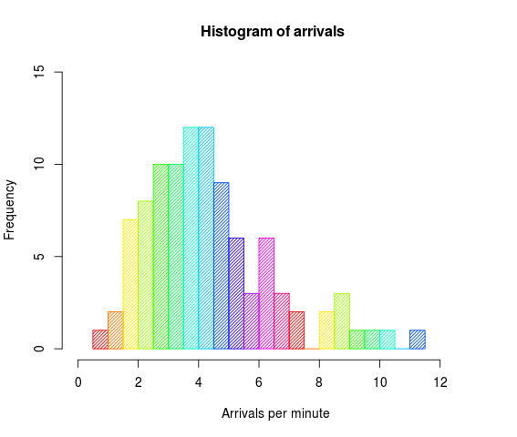
_{[image credits: DanielPenfield (CC BY-SA 3.0)]}

By getting such a distribution for both a potential signal and the background, one can further decide whether this variable could be of any use to increase the signal-over-background ratio (that is the goal of any LHC analysis).

MadAnalysis 5 comes with varied methods making histogramming easy. The procedure is the folllowing.

1- In the Initialize method of the analysis, one needs to declare a signal region by adding

  Manager()->AddRegionSelection(“dummy”);

I intentionally skip any detail about that, as this will be addressed in 2 or 3 posts.

2- Still in the Initialize method, one needs to declare the histogram we would like to show,

  Manager()->AddHisto("ptj1",15,0,1200);

This declares a histogram named ptj1, containing 15 bins ranging from 0 to 1200.

3- At the beginning of the Execute method, one needs to read of the weight of each event, as not all events are necessarily equal,

  Manager()->InitializeForNewEvent(event.mc()->weight());

Those weight will be accounted for when the histogram will be filled, each event therefore entering with the adequate weight.

4- Finally, one still need to fill out histogram, in the Execute method,

  Manager()->FillHisto("ptj1”,10.)

The first argument refers to the name of the histogram, and the second one is the value.

5- After running the code on an input file named tth.list, the output file is Output/tth/test_analysis_X/Histograms/histos.saf where the capital X is a number increased every time the code is run. Each declared histogram is present in this XML-like file, within a given <Histo> element,

For a given histograms, one can find information about the number of bins and the range,

  # nbins   xmin           xmax
     15      0.000000e+00   1.200000e+03

some statistics and the value of each bin

   <Data>
       0.000000e+00   0.000000e+00    # underflow
       0.000000e+00   0.000000e+00    # bin 1 / 15
       3.639279e-04   0.000000e+00    # bin 2 / 15
       2.362230e-04   0.000000e+00
      …
  </Data>

The total value corresponding to each bin is obtained from the sum of the numbers of the two columns. Once again, I will skip any detail concerning the reason behind that;)

A FIRST MADANALYSIS 5 TASK REQUEST

Completely unrelated to the rest, there is no dedicated module allowing one to read a histos.saf file and get plots out of it. I would like to get a Python code (potentially relying on matplotlib) allowing to do so. An exemplary histogram file can be found here.

This will be the first task request of this particle physics @ utopian-io project. Please do not forget to mention me in any post detailing such an implementation.

The deadline is Friday June 29th, 16:00 UTC.

THE EXERCISE

For the exercise of the day, we will move away from our previous analysis and start the study of a CMS search for dark matter. We will come back to the ATLAS analysis in the future.

As usual, one should avoid implementing every single line in the analysis and follow instead the instructions below. Please do not hesitate to shoot questions in the comments.

Create a blank analysis from the MadAnalysis 5 main folder,
./bin/ma5 -E test_cms test_cms
We will modify the file test_cms/Build/SampleAnalyzer/User/Analyzer/test_cms.cpp below.
In the Initialize method of this file, please declare a dummy signal region (see above),
Manager()->AddRegionSelection("dummy");
In the Execute method of this file, initialize the weights (in the aim of getting histograms),
Manager()->InitializeForNewEvent(event.mc()->weight());
Go to section 3 of the CMS analysis note, on page 4. Create a vector with signal jets as described in the middle of the second paragraph. This is similar to anything we have done so far, as we only focus on transverse momentum and pseudorapidity constraints here.
Go the third paragraph on page 3 and create a vector containing all (isolated) signal photons. There is no transverse momentum requirement on the photons, but a pseudorapidity one (see in the second paragraph of section 3 on page 4). Isolation has to be implemented as described above, the thresholds being given in the medium barrel information of table 3 in this research paper. Whilst the σ_ηη criterion can be ignored, the requirement on H/E can be implemented thanks to the HEoverEE() method of the RecPhotonFormat class.
Implement four histograms of 20 bins each. Two of them will be related to the transverse momentum of the first photon and of the first jet, both covering a p_T range from 0 to 1000 GeV. The last two histograms will be related to the pseudorapidity spectra of the same objects, covering the [-1.5,1.5] range for the first photon and the [-5,5] range for the first jet.
Apply the code on the previous sample of 10 simulated LHC collisions (see here).

Don’t hesitate to write a post presenting and detailing your code. Note that posts tagged with utopian-io tags as the first two tags (and steemstem as a third) will be reviewed independently by steemstem and utopian-io. Posts that do not include the utopian-io tags as the first two tags will not be reviewed by the utopian-io team.

The deadline is Friday June 29th, 16:00 UTC.

MORE INFORMATION ON THIS PROJECT

The idea
The project roadmap
Step 1a: implementing electrons, muons and photons
Step 1b: jets and object properties
Step 1c: isolation and histograms (this post)

Participant posts (alphabetical order):

@effofex: exercise 1b, madanalysis 5 on windows 10
@irelandscape: journey through particle physics (1, 2, 2b, 3), exercise 1b, exercise 1a
@mactro: exercise 1b, exercise 1a.

STEEMSTEM

SteemSTEM is a community-driven project that now runs on Steem for more than 1.5 year. We seek to build a community of science lovers and to make the Steem blockchain a better place for Science Technology Engineering and Mathematics (STEM).

More information can be found on the @steemstem blog, on our discord server and in our last project report. Please also have a look on this post for what concerns the building of our community.

Particle physics @ utopian-io - Objects isolation, histogramming and a first task request